13. Image preprocessing
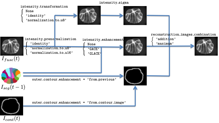
Fig. 13.1 Pre-processing of fusion images.
The segmentation process involves 3 valued (or grey-level) images:
the so-called seed image for the computation of \(h\)-minima to extract seeds (see sections Step 2: seed extraction and Step 2: \hat{S}_{t})
the so-called membrane image used as the elevation map for the computation of the seeded watershed (see sections Step 5 : seeded watershed, Step 1: \tilde{S}_{t}, and Step 2: \hat{S}_{t})
the image for the morphosnake correction (see section Steps 5 and 6: morphosnake correction)
These images may be transformed version of the fused image: figure Pre-processing of fusion images. presents the workflow to obtain these images.
First, the values (or intensities) of the fused image may be normalized into 1 or 2 unsigned byte(s),
depending on the value of intensity_prenormalization. This first normalization has been
introduced to deal with floating encoded images, and should not be used for images already
encoded on 1 or 2 unsigned byte(s)
Second, this pre-normalized image can undergo 3 different processing, and the resulting image will be a combination of this 3 images.
intensity_transformationtransform the image values based on its histogram and allows to normalize the intensities of the input image into 1 or 2 unsigned byte(s), either globally or an a cell basis (only in segmentation propagation). This image can be further smoothed by a gaussian kernel (ifintensity_sigma> 0). See section Histogram based image value transformation.intensity_enhancementtransform the image based on a membrane dedicated process, either globally or an a cell basis, which requires the previous segmentation (only in segmentation propagation then). See section Membrane dedicated enhancement.outer_contour_enhancementadds a fake outer membrane, either issued from the previous segmentation (only in segmentation propagation then) or given as input images (see section Preprocessing parameters).
The combination mode is set by the reconstruction_images_combination variable.
If the fused image is transformed before being segmented, the
transformed image is named <EN>_xxx_t<timepoint>.<image_suffix>
(with xxx being either membrane, seed, or morphosnake)
and stored in the directory REC-XXX/REC_<EXP_SEG>/ or REC-XXX/REC_<EXP_RECONSTRUCTION>/
with
XXXbeing eitherMEMBRANE,SEED, orMORPHOSNAKE, andEXP_RECONSTRUCTIONoverridesEXP_SEGif both variables are present in the parameter file.
if the value of the variable keep_reconstruction is set to True.
Only one of them is computed if the pre-processing parameters are the same for the 3 images.
None are computed if the 3 images are equal to the fused images.
Note that specifying
intensity_prenormalization = 'identity'
intensity_transformation = 'identity'
intensity_enhancement = None
outer_contour_enhancement = None
in the parameter file comes to use the unprocessed fused image as input image for seed extraction, watershed, and morphosnake computation.
A comprehensive list of the pre-processing parameters can be found in
section Preprocessing parameters.
Pre-processing parameters can be set differently for the seed, membrane and morphosnake images
by prefixing them (see section Prefixed parameters) by
seed_, membrane_ or morphosnake_
(see sections astec_mars parameters and astec_astec parameters).
13.1. Histogram based image value transformation
The option intensity_transformation can be set to one of the following values.
Nonethis pre-processing channel is not used, meaning that only the membrane dedicated process will produce the input for the segmentation.
'identity'there is no transformation of the fused image.
'normalization_to_u8'input images are usually encoded on 2 bytes. However, it is of some interest to have input images of similar intensity distribution, so the segmentation parameters (eg the \(h\) for the regional minima computation) do not have to be tuned independently for each image or sequence.
This choice casts the input image on a one-byte image (ie into the value range \([0, 255]\)) by linearly mapping the fused image values from \([I_{min}, I_{max}]\) to \([0, 255]\). \(I_{min}\) and \(I_{max}\) correspond respectively to the 1% and to the 99% percentiles of the fused image cumulative histogram. This allows to perform a robust normalization into:math:[0, 255] without being affected by extremely low or high intensity values. Values below \(I_{min}\) are set to \(0\) while values above \(I_{max}\) are set to \(255\).
The percentiles used for the casting can be tuned by the means of two variables
normalization_min_percentile = 0.01
normalization_max_percentile = 0.99
'normalization_to_u16'This is similar to the
'normalization_to_u8'except that the input image is casted on a two-bytes image (ie into the value range [0,normalization_max_value]).
13.2. Membrane dedicated enhancement
The option intensity_enhancement can be set to one out the two (segmentation of the first time point,
see section astec_mars) or three (segmentation by propagation of the other time points,
see section astec_astec) values.
Nonethis pre-processing channel is not used, meaning that only the histogram based image value transformation will produce the input for the segmentation.
'GACE'stands for Global Automated Cell Extractor. This is the method described in [MGFM14], [Mic16].
'GLACE'stands for Grouped Local Automated Cell Extractor. It differs from one step from
GACE: the threshold of extrema image is not computed globally (as inGACE), but one threshold is computed per cell of \(S^{\star}_{t-1} \circ \mathcal{T}_{t-1 \leftarrow t}\), from the extrema values of the cell bounding box.
GACE and GLACE consist both of the following steps.
Membrane dedicated response computation. The Hessian is computed by convolution with the second derivatives of a Gaussian kernel (whose standard deviation is given by
mars_sigma_membrane). The analysis of eigenvalues and vectors of the Hessian matrix allows to recognize the normal direction of an eventual membrane. A response is then computed based on a contour detector in the membrane normal direction.Directional extrema extraction. Extrema of the response in the direction of the membrane normal are extracted. It yields a valued image of membrane centerplanes.
Direction dependent automated thresholding.
It has been observed that the membrane contrast depends on the membrane orientation with respect to the microscope apparatus. Directional response histogram are built and a threshold is computed for each of them, which allows to compute a direction-dependent threshold.
Thresholds are computing by fitting known distribution on histograms. Fitting is done by the means of an iterative minimization, after an automated initialization. The sensitivity` option allows to control the threshold choice after the distribution fitting.
Setting the
manualparameter toTrueallows to manually initialize the distribution before minimization thanks to themanual_sigmaoption.Last, the user can directly give the threshold to be applied (this is then a global threshold that did not depend on the membrane direction) by setting the
hard_thresholdingoption atTrue: the threshold to be applied has to set at thehard_thresholdoption.
Sampling. Points issued from the previous binarization step will be further used for a tensor voting procedure. To decrease the computational cost, only a fraction of the binary membrane may be retained. This fractions is set by the
sampleoption.Note
Sampling is performed through pseudo-random numbers. To reproduce a segmentation experiment by either
GACEorGLACE, the random seed can be set thanks to themars_sample_random_seedoption.If one want to reproduce segmentation experiments, the verboseness of the experiments has to be increased by adding at least one
-vin the command line of eitherastec_marsotastec_astec. This ensures that the necessary information will be written into the.logfile. Then, to reproduce one given experiment, one has to retrieve the used random seed'RRRRRRRRRR'from the lineSampling step : random seed = RRRRRRRRRR
in the log file
SEG/SEG_<EXP_SEG>/LOGS/astec_mars-XXXX-XX-XX-XX-XX-XX.logorSEG/SEG_<EXP_SEG>/LOGS/astec_astec-XXXX-XX-XX-XX-XX-XX.log, and then to add the linesample_random_seed = 'RRRRRRRRRR'
in the parameter file to get the same sampling.
Tensor voting. Each retained point of the binary image (together with its membrane normal direction) generates a tensor voting field, whose extent is controlled by the
sigma_TVoption (expressed in voxel units). These fields are added to yield a global tensor image, and a membraness value is computed at each point, resulting in a scalar image.Smoothing. An eventual last smoothing of this scalar image may be done, controlled by the
sigma_LFoption.
13.3. Outer contour
The outer membrane of cells (the one shared with the background) may be
less marked/intense than the one between two cells, thus may cause some segmentation errors.
To alleviate this drawback, a fake contour image can be fused with the transformed image
with the option outer_contour_enhancement can be set to one of the following values.
NoneNo fake outer contour is used.
'from_previous_segmentation'Contour images are built from the previous segmented time point. Fragile. Kept for test purposes. Obviously, works only for propagated segmentation. This feature has been added for tests, but has not demonstrated yet any benefit.
'from_contour_image'Contours images named
<EN>_contour_t<begin>.<image_suffix>are provided in a separate directory<PATH_EMBRYO>/CONTOUR/CONTOUR_<EXP_CONTOUR>/
13.4. Some examples
Here, we have images to be segmented, typically issued from the fusion step (astec_fusion). These images are usually encoded on two (signed or unsigned) bytes, then with values that can go beyond 255.
If keep_reconstruction is set to True, the experiment directory will look like above after
some segmentation step (astec_mars or astec_astec).
/path/to/experiment/
├── ...
├── FUSE/
│  └── FUSE_<EXP_FUSE>/
│     ├── ...
│     ├── <EN>_fuse_t<ttt>.<image_suffix>
│     ├── ...
│     └── LOGS/
├── REC-MEMBRANE/
│  └── REC_<EXP_SEG>
│     ├── ...
│     ├── <EN>_membrane_t<ttt>.<image_suffix>
│     └── ...
├── REC-SEED/
│  └── REC_<EXP_SEG>
│     ├── ...
│     ├── <EN>_seed_t<ttt>.<image_suffix>
│     └── ...
├── SEG/
│  └── SEG_<EXP_SEG>
│      └── ...
...
13.4.1. intensity_transformation = ‘identity’ and intensity_enhancement = None
intensity_transformation = 'identity'
intensity_enhancement = None
The fusion image is not normalized
There is no membrane enhancement
Reconstruction images will be encoded on two (signed or unsigned) bytes (as the fusion ones).
There may be both membrane and seed reconstructed images
if intensity_sigma (see Preprocessing parameters) is set at different values for the two
reconstruction schemes.
13.4.2. intensity_transformation = ‘normalization_to_u8’ and intensity_enhancement = None
intensity_transformation = 'normalization_to_u8'
intensity_enhancement = None
The fusion image is normalized on 1 byte (thus in [0, 255])
There is no membrane enhancement
Reconstruction images will be encoded on one byte.
13.4.3. intensity_transformation = ‘identity’ and intensity_enhancement = ‘gace’
intensity_transformation = 'identity'
intensity_enhancement = 'gace'
The fusion image is not normalized
There is some membrane enhancement. Result image in encoded on one byte, ie in [0, 255]
The reconstruction image will be a combination of the fusion image and the membrane enhanced one. Since the fusion image is encoded on 2 bytes, the reconstruction images will be encoded on two bytes too.
reconstruction_images_combination = 'maximum'. The combination is done by computing the maximum values between the fusion image and the membrane enhanced one. Since the fusion image is on two bytes (with values beyond 255) and the membrane enhanced one is on one byte (in [0, 255]), membrane enhanced values may be always lower than the fusion one, and the reconstruction images are likely to be very similar (if not equal) to the fusion one.reconstruction_images_combination = 'addition'. The combination is done by adding the values of the fusion image and the membrane enhanced one.
13.4.4. intensity_transformation = ‘normalization_to_u8’ and intensity_enhancement = ‘gace’
intensity_transformation = 'normalization_to_u8'
intensity_enhancement = 'gace'
The fusion image is normalized on 1 byte (thus in [0, 255])
There is some membrane enhancement. Result image in encoded on one byte, ie in [0, 255]
The reconstruction image will be a combination of the fusion image and the membrane enhanced one.
reconstruction_images_combination = 'maximum'. Both images to be fused are on one byte (in [0, 255]), thus the resulting image is also in [0, 255] and then encoded on one byte.reconstruction_images_combination = 'addition'. The combination is done by adding the values of the fusion image and the membrane enhanced one. The result in on two bytes.
13.4.5. intensity_transformation = None and intensity_enhancement = ‘gace’
intensity_transformation = None
intensity_enhancement = 'gace'
The fusion image is not directly used
There is some membrane enhancement. Result image in encoded on one byte, ie in [0, 255]
The reconstruction image will be the membrane enhanced one, thus encoded on one byte. Since the membrane enhanced image is 0 apart at the membrane location, extracting (regional) maxima for watershed may be not efficient.