5. astec_fusion
5.1. Fusion method overview
The fusion is made of the following steps.
Optionally, a slit line correction. Some Y lines may appear brighter in the acquisition and causes artifacts in the reconstructed (i.e. fused) image. By default, it is not done.
A change of resolution in the X and Y directions only (Z remains unchanged). It allows to decrease the data volume (and then the computational cost) if the new pixel size (set by
target_resolution) is larger than the acquisition one.Optionally, a crop of the resampled acquisitions. It allows to decrease the volume of data, hence the computational cost. The crop is based on the analysis of a MIP view (in the Z direction) of the volume, and thus is sensitive to hyper-intensities if any. By default, it is done.
Optionally, a mirroring of the images:
if the
acquisition_mirrorsvariable is set toFalse, a mirroring along the X axis of the right camera images (see also section Important parameters in the parameter file), andif the
acquisition_leftcamera_z_stackingvariable is set to'inverse', a mirroring along the Z axis of both left camera and right camera images (see also section Important parameters in the parameter file).
Co-registration of the 3 last images onto the first one (the acquisition from the left camera for stack #0) considered as a reference. The reference image is resampled again, to get an isotropic voxel (whose size is given by
target_resolution), i.e. the voxel size is the same along the 3 directions: X, Y, Z. There are two alternative methods.The direct fusion method. Each of the 3 last images is linearly co-registered onto the reference image.
The hierarchical method. Each stack is first reconstructed (with the acquisition couple of both left and right cameras), then stack #1 is non-linearly co-registered onto stack #0. From this last registration, non-linear co-registrations are deduced for the stack #1 acquisitions, while linear co-registration is still considered for the right camera acquisition of stack #0.
Weighted linear combination of images.
Optionally, a crop of the fused image, still based on the analysis of a MIP view (in the Z direction). By default, it is done.
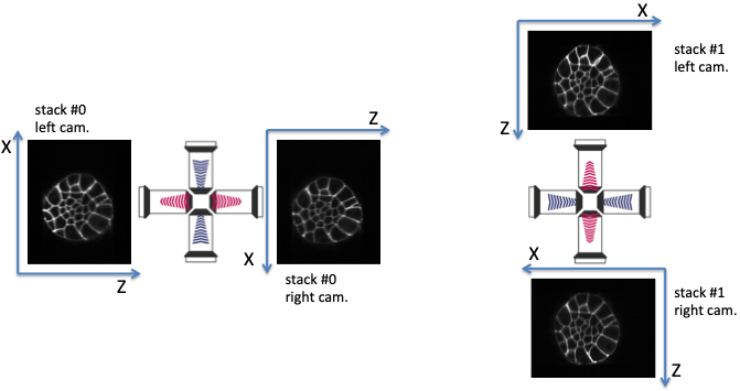
Fig. 5.1 Multiview lightsheet microscope acquisition (‘right’ acquisition).
Multiview lightsheet microscope acquisition: at a time point, two acquisitions (stack #0 and stack #1) are sequentially performed, the second one orthogonal to the first. For each acquisition, two 3D intensity image stacks are acquired, respectively by the left and the right cameras. It yields four image stacks to be fused. The frame (X,Z) of the left camera of stack #0 needs to be rotated clockwise (90 degrees along the Y axis) to correspond to the frame of the left camera of stack #1: acquisition_orientation has to be set to 'right' if acquisition_leftcamera_z_stacking is set to 'direct'.
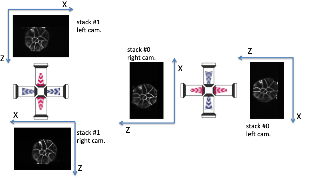
Fig. 5.2 Multiview lightsheet microscope acquisition (‘left’ acquisition).
The frame (X,Z) of the left camera of stack #0 needs to be rotated counterclockwise (-90 degrees along the Y axis) to correspond to the frame of the left camera of stack #1: acquisition_orientation has to be set to 'left' if acquisition_leftcamera_z_stacking is set to 'direct'.
5.2. Important parameters in the parameter file
A simple parameter file for fusion is described in the tutorial section. An exhaustive presentation of all parameters can be found in section astec_fusion parameters.
Indicating the right values of the acquisition parameters is crucial; these parameters are
acquisition_mirrors(orraw_mirrors) is a parameter indicating whether the right camera images have already been mirrored along the X axis (so that the X axis direction is the one of the left cameras) or not. Its value is eitherFalseorTrue. Such a parameter should depend on the acquisition apparatus (ie the microscope) and the should be identical for all acquisitions.In acquisitions depicted in figures Multiview lightsheet microscope acquisition (‘right’ acquisition). and Multiview lightsheet microscope acquisition (‘left’ acquisition)., it can be seen that the X-axis of the right camera image is inverted with respect to the left camera image.
acquisition_mirrorshas to be set toFalse.acquisition_orientation(orraw_ori) is a parameter describing the acquisition orientation of the acquisition of the stack #1 images with respect to the stack #0 ones.'right': the frame (X, Z) of the left camera of stack #0 needs to be rotated clockwise (90 degrees along the Y axis) to correspond to the left camera of stack #1 (see figure Multiview lightsheet microscope acquisition (‘right’ acquisition).).'left': the frame (X, Z) of the left camera of stack #0 needs to be rotated counterclockwise (-90 degrees along the Y axis) to correspond to the left camera of stack #1 (see figure Multiview lightsheet microscope acquisition (‘left’ acquisition).).
acquisition_leftcamera_z_stackinggives the order of stacking of in the Z direction for the left camera images.'direct': z increases from the high-contrasted images to the blurred ones (see figure Multiview lightsheet microscope acquisition (‘right’ acquisition).).'inverse': z increases from the blurred images to the high-contrasted ones (see figure Multiview lightsheet microscope acquisition (‘left’ acquisition).).
Looking at XZ-sections of the registered images (see figures Fusion with constant weighting function., Fusion with ramp weighting function., Fusion with corner weighting function., and Fusion with Guignard’s weighting function.) provides an efficient means to check whether this parameter is correctly set (see also section Step 6: linear combination of co-registered image stacks).
acquisition_resolution(orraw_resolution) is the voxel size (along the 3dimensions X, Y and Z) of the acquired images.
target_resolutionis the desired isotropic (thesame along the 3 dimensions) voxel size for the result fusion images.
begingives the index of the first time point to be processed.endgives the index of the last time point to be processed.
When one may not be sure of the raw_ori, raw_mirrors, and acquisition_leftcamera_z_stacking right values, it is advised to perform the
fusion on only one time point (by indicating the same index for both
begin and end), e.g. with the four possibilities for the
variable couple (raw_ori, raw_mirrors), i.e. ('left', False),
('left', True), ('right', False), and ('right', True).
It comes to write four parameter files that differ only for the
parameters raw_ori, raw_mirrors, and EXP_FUSE (to store the fusion result in different directories, see section Fusion / output data).
For these first experiments, it is advised
to set
target_resolutionto a large value, in order to speed up the calculations, andto set
fusion_xzsection_extractiontoTrue(or some adequate value), in order to check whetheracquisition_leftcamera_z_stackingwas correctly set (see also section Step 6: linear combination of co-registered image stacks).
Please recall that raw_ori should depend on the acquisition apparatus (ie the microscope), and should not change for all the other acquisitions on the same microscope (unless the microscope settings change). Then, for most experiments, one change only to test the value of
raw_ori.
Please note that changing the value of acquisition_leftcamera_z_stacking implies to change also the value of acquisition_orientation.
5.3. Fusion / input data
Input data (acquired images from the MuViSPIM microscope, see figures Multiview lightsheet microscope acquisition (‘right’ acquisition). and Multiview lightsheet microscope acquisition (‘left’ acquisition).) are assumed
to be organized in a separate RAWDATA/ directory in the
/path/to/experiment/ directory as depicted below.
RAWDATA/LC/Stack0000contains the images acquired at the first angulation by the left camera.RAWDATA/LC/Stack0001contains the images acquired at the second angulation by the left camera.RAWDATA/RC/Stack0000contains the images acquired at the first angulation by the right camera.RAWDATA/RC/Stack0001contains the images acquired at the second angulation by the right camera.
/path/to/experiment/
├── RAWDATA/
│  ├── LC/
│  │  ├── Stack0000/
│  │  │   ├── Time000xxx_00.zip
│  │  │   ├── ...
│  │  │   └── Time000xxx_00.zip
│  │  └── Stack0001/
│  │     ├── Time000xxx_00.zip
│  │     ├── ...
│  │     └── Time000xxx_00.zip
│  └── RC/
│     ├── Stack0000/
│     │   ├── Time000xxx_00.zip
│     │   ├── ...
│     │   └── Time000xxx_00.zip
│     └── Stack0001/
│        ├── Time000xxx_00.zip
│        ├── ...
│        └── Time000xxx_00.zip
...
where xxx denotes a three digit number (e.g. 000, 001, …) denoting the time point of each acquisition. The range of time points to be fused are given by the variables begin and end, while the path /path/to/experiment/ has to be assigned to the variable PATH_EMBRYO.
Hence a parameter file containing
PATH_EMBRYO = /path/to/experiment/
begin = 0
end = 10
indicates that time points in [0,10] of the RAWDATA/ subdirectory of /path/to/experiment/ have to be fused.
5.3.1. Input data directory names
However, directories may be named differently. The variables
DIR_RAWDATA, DIR_LEFTCAM_STACKZERO, DIR_RIGHTCAM_STACKZERO, DIR_LEFTCAM_STACKONE, and DIR_RIGHTCAM_STACKONE allow a finer control of the
directory names. The images acquired at the first angulation by the
left and the right cameras are searched in the directories
<PATH_EMBRYO>/<DIR_RAWDATA>/<DIR_LEFTCAM_STACKZERO>
<PATH_EMBRYO>/<DIR_RAWDATA>/<DIR_RIGHTCAM_STACKZERO>
while the images acquired at the second angulation by the left and the right cameras are searched in the directories
<PATH_EMBRYO>/<DIR_RAWDATA>/<DIR_LEFTCAM_STACKONE>
<PATH_EMBRYO>/<DIR_RAWDATA>/<DIR_RIGHTCAM_STACKONE>
where <XXX> denotes the value of the variable XXX.
Then, to parse the following data architecture
/path/to/experiment/
├── my_raw_data/
│  ├── LeftCamera/
│  │  ├── FirstStack/
│  │  │   └── ...
│  │  └── SecondStack/
│  │     └── ...
│  └── RightCamera/
│     ├── FirstStack/
│     │   └── ...
│     └── SecondStack/
│        └── ...
...
one has to add the following lines in the parameter file
DIR_RAWDATA = 'my_raw_data'
DIR_LEFTCAM_STACKZERO = 'LeftCamera/FirstStack'
DIR_RIGHTCAM_STACKZERO = 'RightCamera/FirstStack'
DIR_LEFTCAM_STACKONE = 'LeftCamera/SecondStack'
DIR_RIGHTCAM_STACKONE = 'RightCamera/SecondStack'
It has to be noted that, when the stacks of a given time point are in different directories, image file names are tried to be guessed from the directories parsing. It has to be pointed out that indexes have to be encoded with a 3-digit integer with 0 padding (i.e. 000, 001, …) and that has to be the only variation in the file names (within each directory).
5.3.2. Input data image file names
Images acquired from the left and the right cameras may be stored in the same directory, but obviously with different names as in
/path/to/experiment/
├── RAWDATA/
│  ├── stack_0_channel_0/
│  │  ├── Cam_Left_00xxx.zip
│  │  ├── ...
│  │  ├── Cam_Right_00xxx.zip
│  │  └── ...
│  └── stack_1_channel_0/
│     ├── Cam_Left_00xxx.zip
│     ├── ...
│     ├── Cam_Right_00xxx.zip
│     └── ...
...
The parameter file has then to contain the following lines to indicate the directory names.
DIR_LEFTCAM_STACKZERO = 'stack_0_channel_0'
DIR_RIGHTCAM_STACKZERO = 'stack_0_channel_0'
DIR_LEFTCAM_STACKONE = 'stack_1_channel_0'
DIR_RIGHTCAM_STACKONE = 'stack_1_channel_0'
In addition, to distinguish the images acquired by the left camera to
those acquired by the right one, one has to give the image name
prefixes, i.e. the common part of the image file names before the
3-digit number that indicates the time point.
This is the purpose of the variables acquisition_leftcam_image_prefix and acquisition_rightcam_image_prefix.
The parameter file has then to contain the following lines not only to indicate
the directory names but also the image file name prefixes.
DIR_LEFTCAM_STACKZERO = 'stack_0_channel_0'
DIR_RIGHTCAM_STACKZERO = 'stack_0_channel_0'
DIR_LEFTCAM_STACKONE = 'stack_1_channel_0'
DIR_RIGHTCAM_STACKONE = 'stack_1_channel_0'
acquisition_leftcam_image_prefix = 'Cam_Left_00'
acquisition_rightcam_image_prefix = 'Cam_Right_00'
5.3.3. Fusion / input data / multichannel acquisition
In case of multichannel acquisition, the fusion is computed for the first channel, and the computed parameters (e.g. transformations, etc.) are also used for the other channels.
For a second channel, the images acquired at the first angulation by the left and the right cameras are searched in the directories
<PATH_EMBRYO>/<DIR_RAWDATA>/<DIR_LEFTCAM_STACKZERO_CHANNEL_1>
<PATH_EMBRYO>/<DIR_RAWDATA>/<DIR_RIGHTCAM_STACKZERO_CHANNEL_1>
while the images acquired at the second angulation by the left and the right cameras are searched in the directories
<PATH_EMBRYO>/<DIR_RAWDATA>/<DIR_LEFTCAM_STACKONE_CHANNEL_1>
<PATH_EMBRYO>/<DIR_RAWDATA>/<DIR_RIGHTCAM_STACKONE_CHANNEL_1>
For a third channel, the images acquired at the first angulation by the left and the right cameras are searched in the directories
<PATH_EMBRYO>/<DIR_RAWDATA>/<DIR_LEFTCAM_STACKZERO_CHANNEL_2>
<PATH_EMBRYO>/<DIR_RAWDATA>/<DIR_RIGHTCAM_STACKZERO_CHANNEL_2>
while the images acquired at the second angulation by the left and the right cameras are searched in the directories
<PATH_EMBRYO>/<DIR_RAWDATA>/<DIR_LEFTCAM_STACKONE_CHANNEL_2>
<PATH_EMBRYO>/<DIR_RAWDATA>/<DIR_RIGHTCAM_STACKONE_CHANNEL_2>
5.4. Fusion / output data
The variable target_resolution allows to set the desired isotropic (the
same along the 3 dimensions) voxel size for the result fusion
images.
5.4.1. Output data directory names
The resulting fused images are stored in sub-directory FUSE/FUSE_<EXP_FUSE> under the /path/to/experiment/ directory
/path/to/experiment/
├── RAWDATA/
│  └── ...
├── FUSE/
│  └── FUSE_<EXP_FUSE>/
|      ├── LOGS
|      └── ...
...
where <EXP_FUSE> is the value of the variable EXP_FUSE (its
default value is 'RELEASE'). Hence, the line
EXP_FUSE = 'TEST'
in the parameter file will create the directory``FUSE/FUSE_TEST/`` in which the fused images are stored. For instance, when testing for the values of the variable couple
(raw_ori, raw_mirrors), a first parameter file may contain
EXP_FUSE = 'TEST'
raw_ori = 'left'
raw_mirrors = False
begin = 1
end = 1
EXP_FUSE = 'TEST-LEFT-FALSE'
a second parameter file may contain
EXP_FUSE = 'TEST'
raw_ori = 'left'
raw_mirrors = True
begin = 1
end = 1
EXP_FUSE = 'TEST-LEFT-TRUE'
etc. The resulting fused images will then be in different directories.
/path/to/experiment/
├── RAWDATA/
│  └── ...
├── FUSE/
│  ├── FUSE_TEST-LEFT-FALSE/
│  │  └── ...
│  └── FUSE_TEST-LEFT-TRUE/
│     └── ...
...
This will ease their visual inspection to decide which values of the variable couple
(raw_ori, raw_mirrors) to use for the fusion.
The LOGS directory contains an history of all the commands launched, a copy of the parameter files used
(suffixed by date and time), as well as a log file (also suffixed by date and time) of the command execution.
This log file contains the trace written at the console at the time of execution, but also
some additional information which may be useful to diagnose errors.
5.4.2. Output data file names
Fused image files are named after the variable EN:
<EN>_fuse_t<xxx>.<image_suffix> where <xxx> is the time point
index encoded by a 3-digit integer (with 0 padding).
5.4.3. Fusion / output data / multichannel acquisition
If a single name is given in the variable EXP_FUSE, this name will be used to build the directory name for
the resulting fused images of the first channel, and the other directory names are built after this first name by adding a suffix _CHANNEL_2 for the 2nd channel, _CHANNEL_3 for the 3rd channel, etc.
If the parameter file contains
EXP_FUSE = 'MULTI'
The resulting fused images will then be the following directories
/path/to/experiment/
├── RAWDATA/
│  └── ...
├── FUSE/
│  ├── FUSE_MULTI/
│  │  └── ...
│  └── FUSE_MULTI_CHANNEL_2/
│     └── ...
...
Alternatively, a list of names can be specified in the variable EXP_FUSE, these names will be used to build the directory names for
the resulting fused images of the corresponding channels (the first name of the list for the first channel, etc.).
If the parameter file contains
EXP_FUSE = ['1CHANNEL', '2CHANNEL']
The resulting fused images will then be the following directories
/path/to/experiment/
├── RAWDATA/
│  └── ...
├── FUSE/
│  ├── FUSE_1CHANNEL/
│  │  └── ...
│  └── FUSE_2CHANNEL/
│     └── ...
...
5.5. Step 3 parameters: raw data cropping
For computational cost purposes, raw data (images acquired by the MuViSPIM microscope) are cropped (only in X and Y dimensions) before co-registration. A threshold is computed with Otsu’s method [Ots79] on the maximum intensity projection (MIP) image. The cropping parameters are computed to keep the above-threshold points in the MIP image, plus some extra margins. Hyper-intense areas may biased the threshold computation, hence the cropping.
To desactivate this cropping, the line
acquisition_cropping = False
has to be added in the parameter file.
An additional crop along the Z direction can be done by adding
acquisition_z_cropping = True
in the parameter file.
5.6. Step 5 parameters: image co-registration
To fuse the images, they are co-registered onto a reference one. Co-registration are conducted only on the first channel (in case of multiple channel acquisitions), and the computed transformations are also applied onto the other channels. The reference image is chosen as being the acquisition from the left camera for the first stack (also denoted stack #0). The co-registration strategy is given by the variable fusion_strategy in the parameter file.
5.6.1. Fusion direct strategy
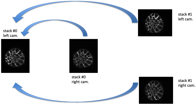
Fig. 5.3 Fusion direct strategy.
Fusion direct strategy: each 3D image is co-registered on the reference one, chosen here as the left camera image of stack #0.
In the parameter file, the line
fusion_strategy = 'direct-fusion'
will set the co-registration strategy to the one described in [Gui15] and [GFL+20]: each acquisition image is linearly co-registered with the reference one, i.e. the one from the left camera and for the first stack.
Let us denote by \(I^{0}_{LC}\) the left camera image of stack #0, the three other images are \(I^{0}_{RC}\), \(I^{1}_{LC}\), and \(I^{1}_{RC}\). By (linear) co-registration (see section Acquisitions linear co-registration) of these image with \(I^{0}_{LC}\), the 3 transformations \(T_{I^{0}_{RC} \leftarrow I^{0}_{LC}}\), \(T_{I^{1}_{LC} \leftarrow I^{0}_{LC}}\), and \(T_{I^{1}_{RC} \leftarrow I^{0}_{LC}}\) are computed. \(T_{I^{0}_{RC} \leftarrow I^{0}_{LC}}\) is the transformation that allows to resample \(I^{0}_{RC}\) in the same frame than \(I^{0}_{LC}\): this transformation goes from the frame of \(I^{0}_{LC}\) towards the frame of \(I^{0}_{RC}\) (hence the direction of the arrow). \(I^{0}_{RC} \circ T_{I^{0}_{RC} \leftarrow I^{0}_{LC}}\) denotes this resampled image.
5.6.2. Fusion hierarchical strategy
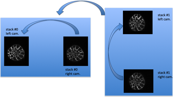
Fig. 5.4 Fusion hierarchical strategy.
Fusion hierarchical strategy. Stacks #0 and #1 are reconstructed independently: right camera images are co-registered on the left camera ones, and stacks #0 and #1 are reconstructed by fusing left and right camera images. Fused image of stack #1 is co-registered on fused image of stack #0: by transformation composition, it allows to compute the transformations of left and right camera images of stack #1 onto the left camera image of stack #0.
In the parameter file, the line
fusion_strategy = 'hierarchical-fusion'
defines a hierarchical co-registration strategy. First, the right camera image of each stack is linearly co-registered (see section Acquisitions linear co-registration) on its left camera counterpart, yielding the transformations \(T_{I^{0}_{RC} \leftarrow I^{0}_{LC}}\) and \(T_{I^{1}_{RC} \leftarrow I^{1}_{LC}}\). According that the left and right camera images of a stack are acquired simultaneously, a linear transformation is then completely adequate to co-register them.
This allows to fuse (see section Step 6: linear combination of co-registered image stacks) the two acquisition of the corresponding left and right cameras into a single stack:
The reconstructed stacks are then (potentially non-linearly, see section Stacks non-linear co-registration) co-registered together, yielding the transformation \(T_{I^{1} \leftarrow I^{0}}\). This allows to get the \(T_{I^{1}_{RC} \leftarrow I^{0}_{RC}}\) and \(T_{I^{1}_{LC} \leftarrow I^{0}_{RC}}\) transformations
Using a non-linear registration in this last step allows to compensate for some distortions that may occur between the two stacks #0 and #1. Please note that stack #0 is then assumed to be the non-distorted reference while left and right camera image of stack #1 will be deformed before fusion.
5.6.3. Acquisitions linear co-registration
The linear co-registrations are either used to co-registered each acquisition onto the reference one in the 'direct-fusion' strategy, or to build stacks from the left and right cameras in the 'hierarchical-fusion' strategy.
Variables that controls the linear co-registrations are either prefixed by fusion_preregistration_ or by fusion_registration_.
To verify whether a good quality registration can be conducted, the searched transformation type can be changed for a simpler one than affine. Adding the following line in the parameter file.
fusion_registration_transformation_type = translation
will search for a translation which could be supposed to be sufficient, according that only translations relates the 4 acquisitions of the MuViSPIM microscope (in a perfect setting). If the search for an affine transformation (the default behavior) failed (the fusion looks poor) while the search for a translation is successful (the fusion looks good), a two-steps registration may help to refine the found translation by a subsequent affine transformation as explained below.
Hyper-intensities areas may bias the threshold calculation used for the automatic crop (step 3 of fusion). In such cases, the iterative registration method may find a local minimum that is not the desired one, because the relative positions of the two images to be co-registered are too far apart. To circumvent such a behavior, a two-steps registration can be done. It consists on a first pre-registration with a transformation with fewer degrees of freedom (i.e. a 3D translation).
This pre-registration can be activated by adding the following line in the parameter file.
fusion_preregistration_compute_registration = True
5.6.4. Stacks non-linear co-registration
Variables that controls the non-linear co-registrations are either prefixed by fusion_stack_preregistration_ or by fusion_stack_registration_. They are defined similarly as the one of acquisitions co-registration.
5.7. Step 6: linear combination of co-registered image stacks
The resampled co-registered image stacks are fused together by the means of a weighted linear combination.
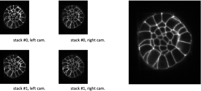
Fig. 5.5 Fusion with constant weighting function.
At the left, XZ-sections of 4 co-registered stacks. At the right, the linear combination of the co-registered stacks with an uniform (or constant) weighting function. It comes to make an average of the 4 co-registered stacks.
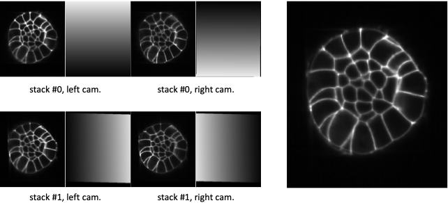
Fig. 5.6 Fusion with ramp weighting function.
At the left, XZ-sections of 4 co-registered stacks together with their ramp weighting function. At the right, the linear combination of the 4 co-registered stacks with this ramp weighting function.
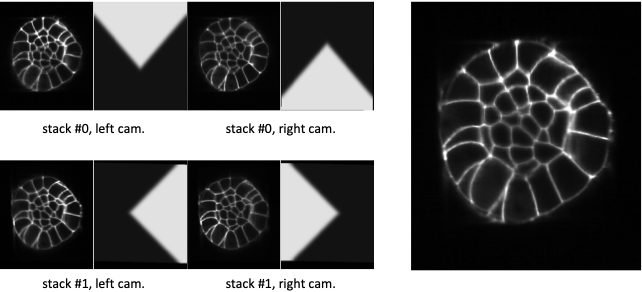
Fig. 5.7 Fusion with corner weighting function.
At the left, XZ-sections of 4 co-registered stacks together with their corner weighting function. At the right, the linear combination of the 4 co-registered stacks with this corner weighting function.
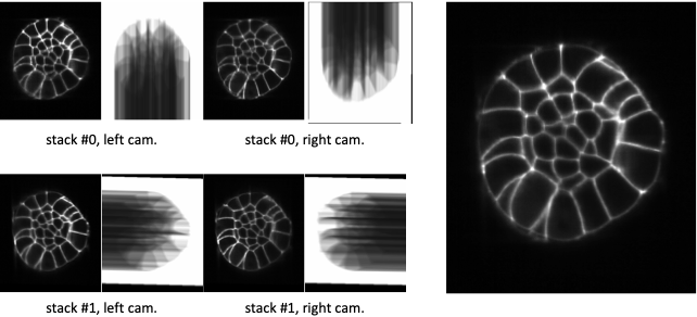
Fig. 5.8 Fusion with Guignard’s weighting function.
At the left, XZ-sections of 4 co-registered stacks together with their Guignard’s weighting function. At the right, the linear combination of the 4 co-registered stacks with this weighting function.
The choice of the weighting function is controlled by the variable fusion_weighting, eventually suffixed by _channel_[1,2,3] if one wants to use different weighting schemes for the different channels to be fused.
The variable fusion_weighting can be set to
'uniform': it comes to the average of the resampled co-registered stacks (see figure Fusion with constant weighting function.). Such a weighting does not depend on the stacks to be fused.'ramp': the weights are linearly increasing along the Z axis (see figure Fusion with ramp weighting function.).'corner': the weights are constant in a corner portion of the stack, defined by two diagonals in the XZ-section (see figure Fusion with corner weighting function.). It somehow mimics a stitching of the 4 resampled co-registered image stacks, where the information is kept from the most informative image.'guignard': the weighting function is the one described in [Gui15]. More weight are given to sections close to the camera and it also takes into account the traversed material (see figure Fusion with Guignard’s weighting function.).
Weighting functions are designed so that the weights decrease with Z for the left camera images and increase with Z for
the left camera images. So, setting the acquisition_leftcamera_z_stacking variable to the wrong value
('direct' instead of 'inverse', or vice-versa) may then decrease the fusion quality.
Looking at XZ-sections of the co-registered image stacks, as well as the weighting function images,
(see figures Fusion with constant weighting function., Fusion with ramp weighting function., Fusion with corner weighting function.,
and Fusion with Guignard’s weighting function.) provides a direct and efficient means to check whether this parameter is
correctly set. Such sections can be extracted by setting the fusion_xzsection_extraction parameter to True
(or some adequate value). It creates XZSECTION_<xxx>/ subdirectories (one per time point, <xxx> being the time
point index) in the FUSE/FUSE_<EXP_FUSE>/ directory.
/path/to/experiment/
├── ...
├── RAWDATA/
│  └── ...
├── FUSE/
│  └── FUSE_<EXP_SEG>/
│     ├── ...
│     ├── XZSECTION_<xxx>/
│     │  └── ...
│     └── ...
...
When using the variable fusion_weighting, the same weights (computed on the first channel to be processed) are used for all fusion. However, different weighting functions can be used for the channels to be fused by using the variables fusion_weighting_channel_[1,2,3], eg
fusion_weighting_channel_1 = 'guignard'
fusion_weighting_channel_2 = 'uniform'
5.8. Step 7: fused data cropping
To save disk storage, fused images are cropped at the end of the fusion stage. To desactivate this cropping, the line
fusion_crop = False
has to be added in the parameter file.
5.9. Troubleshooting
The first step is to parse the log file (see section Fusion / output data) to look for
eventual detected errors.
- The fused images are obviously wrong.
Are the values of the variable couple (
raw_ori,raw_mirrors) the right ones? Conduct experiments as suggested in section Important parameters in the parameter file (see also section Fusion / output data) to get the right values.The registration may have failed.
Try to register with a simpler transformation type (i.e. translation) and/or with a two-steps registration (see section Step 5 parameters: image co-registration).
It also may be due to a cropping failure (see below)
- The imaged sample is cropped by the image border in the fused image.
Check whether the imaged sample was not already cropped in the raw data.
The automated cropping may have failed. Crop borders are indicated in the
logfile and too different crop sizes between the different acquisitions is a cue to diagnose it.
It is more likely to happen when cropping the raw data: to diagnose whether this happens, please see section Step 3: raw data cropping. If it happens, the cropping of raw data can be deactivated (see section Step 3 parameters: raw data cropping). The computational time may however drastically increased. It also may happens that the object of interest (the embryo) is connected to other structures after thresholding: to try to disconnect it, try to perform a morphological opening by setting the variable
acquisition_cropping_openingto a positive value (see also section Step 3: raw data cropping).If it still happens, try to deactivate also the fused image cropping (see section Step 7: fused data cropping).
5.10. Advanced use
Running astec_fusion with the -k option (see section Command line interfaces common options) allows to keep
temporary files. These files are stored in a directory TEMP_<xxx> where xxx denotes a three digit number
(e.g. 000, 001, …) denoting the time point of each acquisition. Since the volume of these is quite large,
the directory is removed after the fusion is completed. However, some of these files may help to diagnose what went
wrong in case of failure. One can use then the -k option, but only to compute a few time points.
/path/to/experiment/
├── ...
├── RAWDATA/
│  └── ...
├── FUSE/
│  └── FUSE_<EXP_SEG>/
│     ├── ...
│     ├── TEMP_<xxx>/
│     │  ├── ANGLE_0
│     │  ├── ANGLE_1
│     │  ├── ANGLE_2
│     │  ├── ANGLE_3
│     │  └── ...
│     └── ...
...
5.10.1. Step 3: raw data cropping
Default cropping of raw data only occurs in the X and Y directions.
This is done by thresholding a maximum intensity projection (MIP), along the Z direction,
of the image after change of resolution (see section Fusion method overview).
The MIP image is thresholded by its average intensity and the largest 4-connected component is kept to compute
the crop borders. This last binary image can be found in the TEMP_<xxx>/ANGLE_<a> directories and is identified
by its suffix _xy_cropselection.
If the variable acquisition_cropping_opening is larger than 0, a morphological opening is performed,
and the resulting binary image is kept with the suffix _xy_open_cropselection. The largest connected component will
afterwards by computed and used to set the crop borders.